A beginner’s guide with R

This guide is intended as a follow-along beginner tutorial that introduces you to to the concepts of an API, what Datawrapper’s API can be used for, and how to get started doing so using R. By the end, you’ll have written the R code to automatically create and publish a Datawrapper line chart with customized settings of your choice, and data pulled automatically from the German Weather Service. You don’t need to have any pre-existing knowledge about R or coding to follow along.

Introduction

What’s an API?

Imagine you're in a library, and you need information from a particular book. Instead of going through the entire library yourself, you ask the librarian for the specific information you need. The librarian knows where to find the book you’re looking for and hands it over to you.

You can think of an API (Application Programming Interface) as a librarian for the internet. It’s a set of rules or instructions (also called protocols) that let different software applications talk to each other and share information or perform actions.

APIs are useful (and powerful, too!) because they allow different programs, websites, or apps to work together and access each other's features or data making things more efficient. For example, imagine you're creating charts for a project. By connecting to an API, you can easily pull in real-time data from other sources, like market trends, and make live-updating charts without the need to manually update the data each time new data comes in.

For a more visual explanation of an API, visit this article on the Datawrapper Blog.

What can you do with Datawrapper's API?

Datawrapper is an online data visualization tool that lets users create interactive and responsive charts, maps, and tables in just a few steps. Datawrapper offers an API that lets you programatically interface with your charts. That means that it lets you create and edit charts, update your account information, get information about which charts you or your team have created, and more —all without the need for manual interaction within the web app interface.

Some scenarios and/or reasons to connect to Datawrapper’s API include:

• scalability: when you need to create loooots of charts
• manipulate external data and create charts with it without the need of having to download any files: for example, you can pull data from the UN’s API and connect to Datawrapper’s API to create a visualization with it
• automation: when you have recurring tasks involving creating new visualizations every x amount of time
• analysis: when you want to get an overview of your or your organization’s usage of Datawrapper

What is DatawRrappr?

To talk to the Datawrapper API, you can choose between many tools. You can connect to the API through a programming language like Python or JavaScript, for example.

For this tutorial, you’ll connect to the API using the R language – and specifically, the R package DatawRrappr, created by Benedict Witzenberger.

He and his package are not connected to Datawrapper, but Benedict did write a guest post for the Datawrapper blog about his R package. Many Datawrapper users make use of the DatawRrappr package to create and edit Datawrapper visualizations from within RStudio.

What is RStudio?

For this tutorial, you can either download and install RStudio or, alternatively, use Posit Cloud. RStudio is an open source software application that lets you run R code. Posit Cloud is an online-based solution that will let you run R code without the need of downloading or installing anything on your laptop.

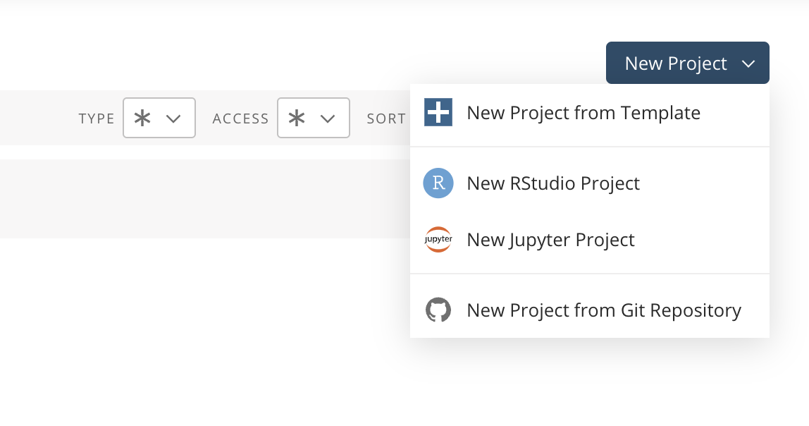
To open a new R project in Posit Cloud, you’ll need to create an account and once you’re logged in, select New Project → New RStudio Project

If you want to start a new R project in the RStudio app, you’ll just need to open the app.

Regardless of which one you choose (RStudio or Posit Cloud), this is what you’ll see:

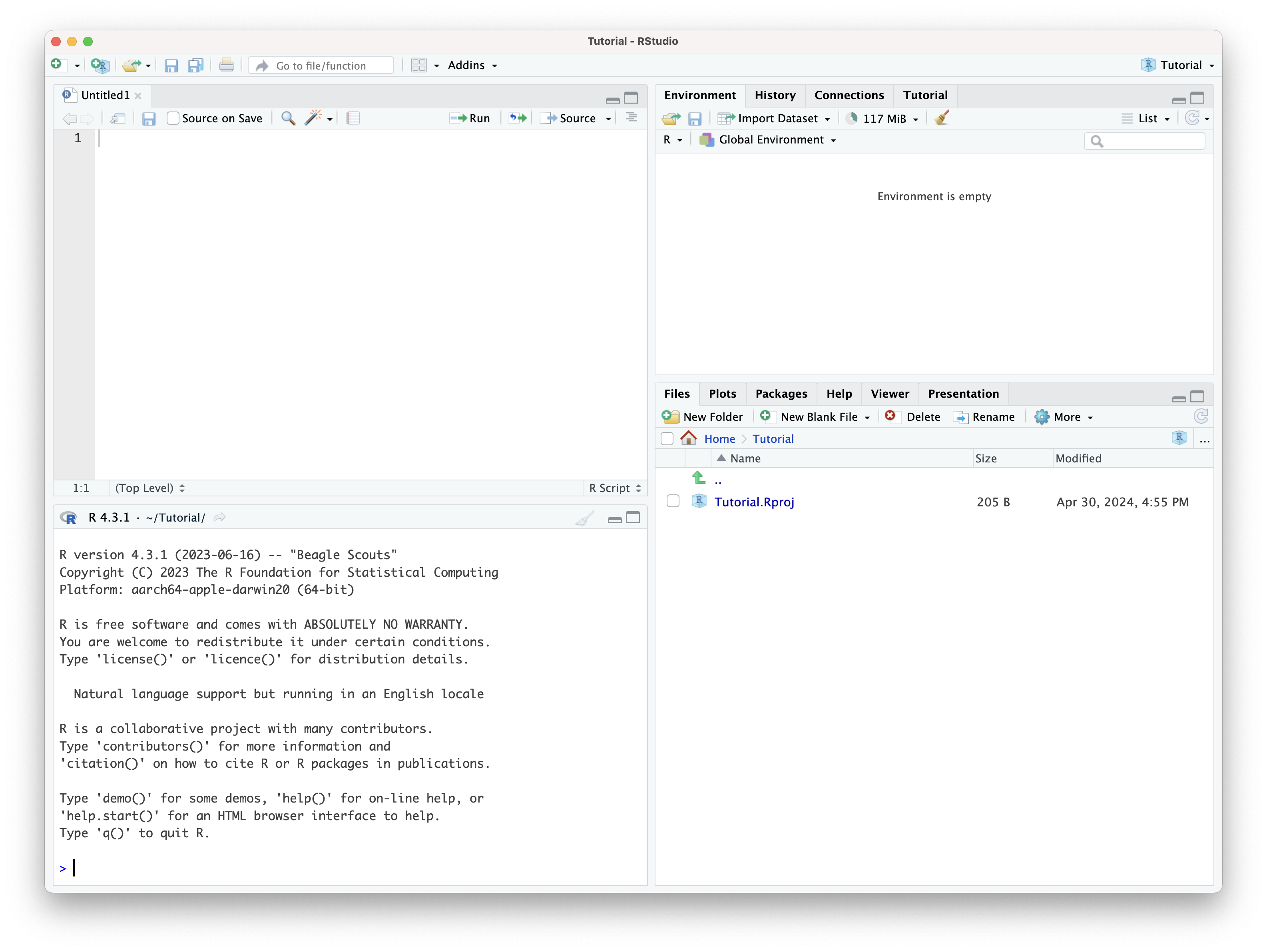
Starting from the bottom left and moving clockwise, the panels are console, source code (where you’ll write the R code), environment, and output:

A step-by-step guide to creating a line chart with Datawrapper's API

Setting up the R environment

Now that you’ve created a new project, next step will be to install the packages you’ll work with. For this tutorial you’ll need the following packages:

• devtools → this package contains useful tools to simplify some tasks in R, like installing packages that live in GitHub for example. (devtools will help us download the datawRappr package from GitHub)
• DatawRappr → this package lets you access the functions in R to talk to Datawrapper’s API and create, refine, publish and re-publish your chart… and more!
• rdwd → this package will let you select, download and read climate data from the German Weather Service. More information on this package here.

Start by installing devtools and DatawRappr. You can do it through Tools > Install Packages… or, alternatively, by calling the packages with the install.packages function.

install.packages("devtools")
devtools::install_github("munichrocker/DatawRappr")
install.packages("rdwd")

Add datawRappr and rdwd to environment.

library(DatawRappr)
library(rdwd)

Try it yourself!

📘

Psst…

You can run R code by…

putting the cursor on the line of the code and then click the Run button at the top of the file window, or…

pressing CTRL (or ⌘) + Enter.

If you want to run multiple lines of code, select the lines you want to run and either click the Run button or press CTRL (or ⌘) + Enter on your keyboard.

💡 As a hint, click on the "R" tab to reveal the code up until this point.

# install packages
install.packages('devtools')
devtools::install_github('munichrocker/DatawRappr')
install.packages('rdwd')

library(DatawRappr)
library(rdwd)

Generating the API key

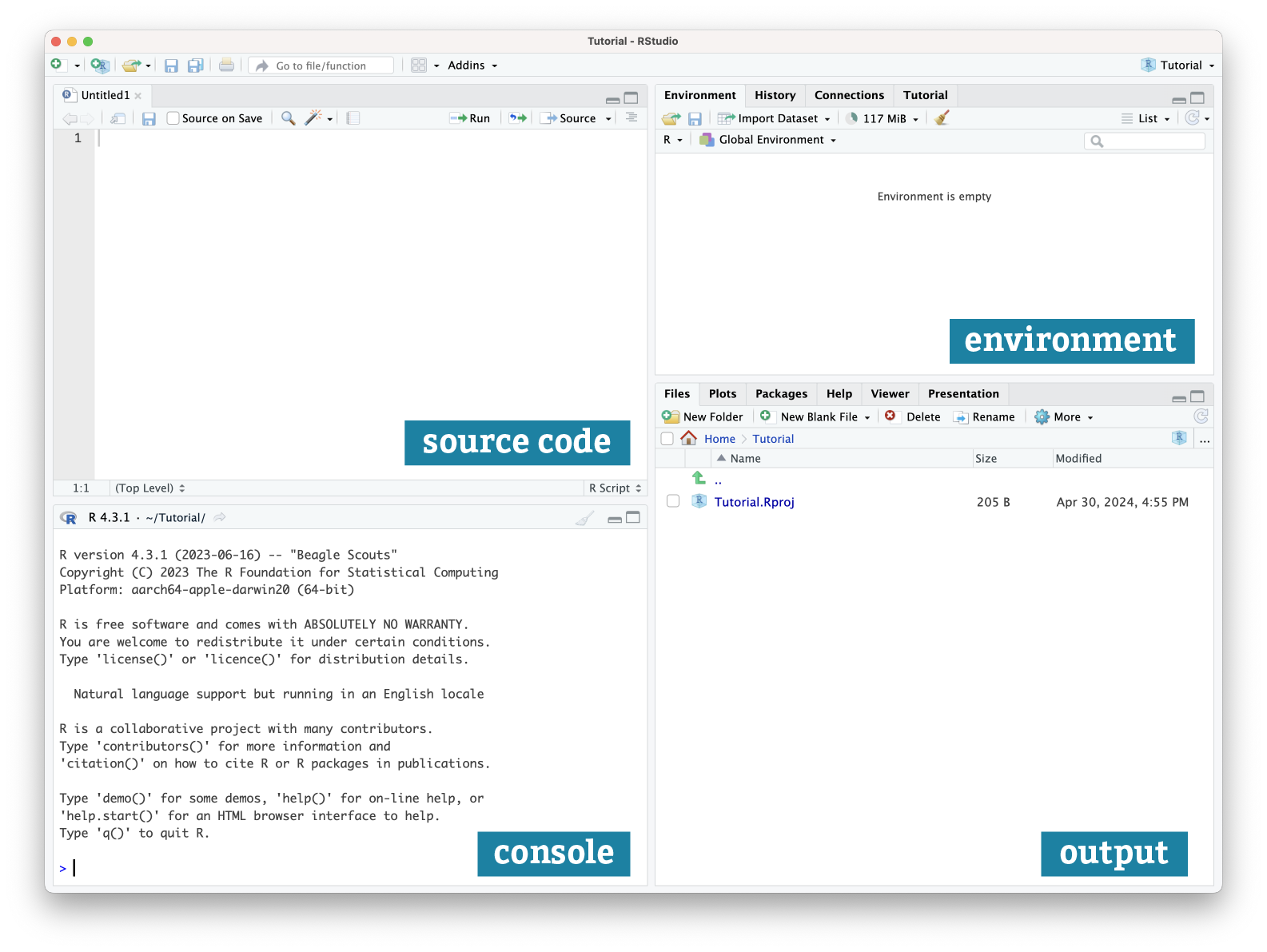
Now that you’ve installed and added the necessary packages to RStudio, you’ll need to create an API access token (think of it as a 🔑). This token is how Datawrapper know it’s you who’s trying to connect to the API. The token is the key to your Datawrapper account that will open the door to creating, publishing, editing visualizations, etc. You can think of this as logging into your Datawrapper account using your login credentials (username and password). To create an access token, you must first create a Datawrapper account (or log in if you already have one!), and then go to your account settings:

Then generate a token with the following permissions:

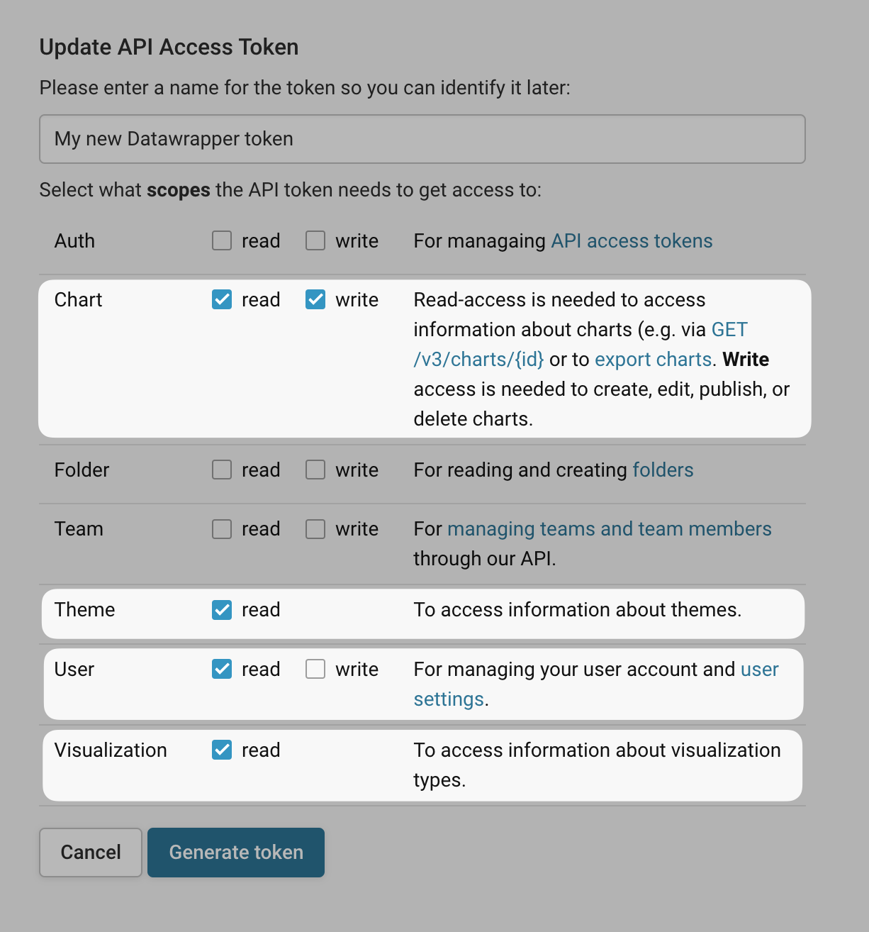
All four scopes chart:read, chart:write, theme:read, and visualization:read are required to publish a chart. And user:read is needed to test the connection to the API. When in doubt, try to always refer to the API documentation.

🚧

Only choose the scope you need, not more.

If your API key gets stolen without you knowing it, you'll be thankful that you didn't give it User or Auth write access. You can still change the scope later with a click on "Edit".

Now that you have the token saved 🔐, you can use it to create an environment where to put it in so that no one can see it. 🙅🏻 

Sys.setenv(DATAWRAPPER_TOKEN = "your token goes here")

Once you create this safe space for your token and run it, you can replace this line of code by actually calling the environment and putting the token to use. To do this, use the first function of the dataWrappr package:

# set the token
datawrapper_auth(api_key = Sys.getenv("DATAWRAPPER_TOKEN"), overwrite = TRUE)

# make sure the key is working as expected
dw_test_key()

After you run dw_test_key() you should get a response from the API indicating whether the connection to the API was successful or not. If it’s successful, the function will return a status code 200. If it wasn’t successful, it will throw an error code. You can refer to the API documentation to learn more about the error codes.

If you got a 200 status code, that’s great! Then you can move on to the next step ✅

💡 As a hint, click on the "R" tab to reveal the code up until this point.

# install packages
install.packages('devtools')
devtools::install_github('munichrocker/DatawRappr')
install.packages('rdwd')

library(DatawRappr)
library(rdwd)

# create an environment for the token 
# (after you run it, you can delete this line) 
Sys.setenv(DATAWRAPPER_TOKEN = "your token goes here")

# set the token
datawrapper_auth(api_key = Sys.getenv("DATAWRAPPER_TOKEN"), overwrite = TRUE)

# make sure the key is working as expected
dw_test_key()

Creating a chart

As a bit of an introduction to DatawRrappr (the R package for Datawrapper) you can head to the documentation and start exploring it. The most important pages for this tutorial are the landing page 🏠 that will walk you through the basics of the package: a brief description, how to install it, its key features, etc., and the Reference page, that contains the details for all functions included in the package.

We’ll start with the dw_create_chart() function. Any function needs some input (argument) to do its job and give you the result you want. In this case, we can pass different arguments into dw_create_chart() to create a chart: api_key, title, type, folderId, and theme.

Let’s create a line chart! 📈 (You could also pick any other chart listed under Chart Types in the package documentation the same way you would do under the Visualize step in the Datawrapper web app).

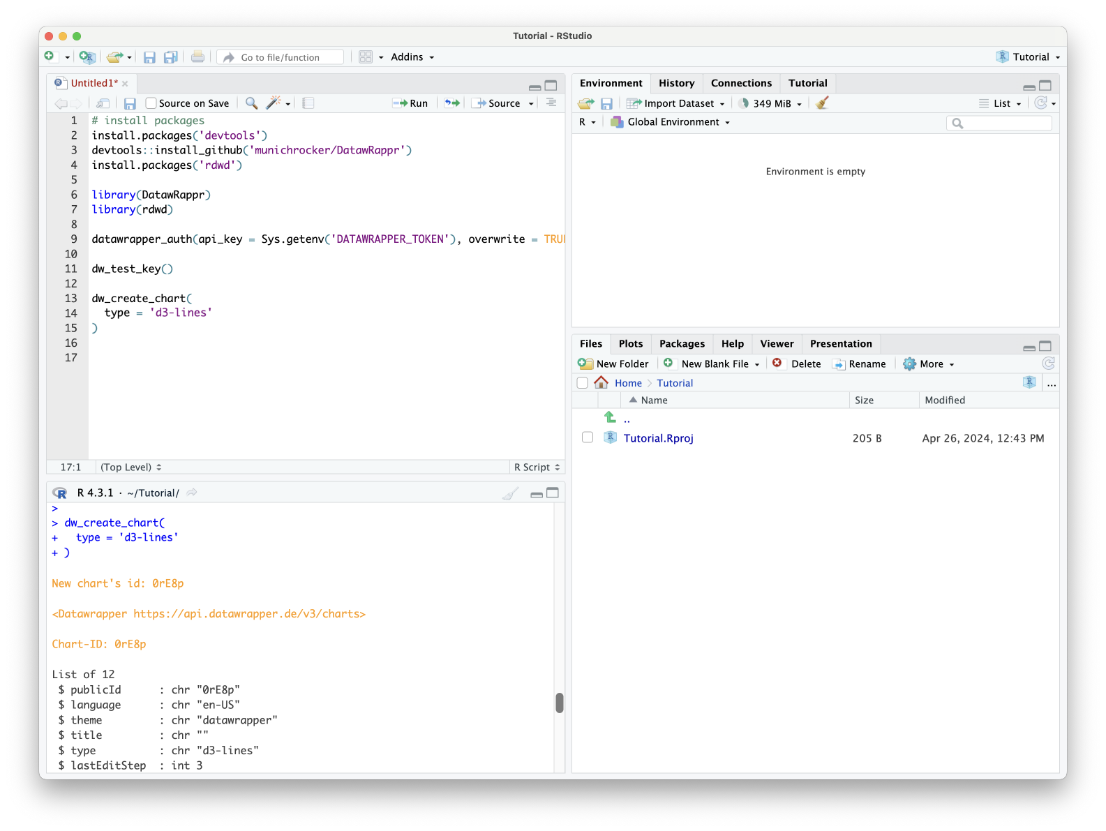
dw_create_chart(        
	type = 'd3-lines'
)

If you run that script, the function will return a chart ID as well as the metadata of the chart in the console. It will look something similar to this:

⭐

Bonus points for...

Can you create a scatter plot?

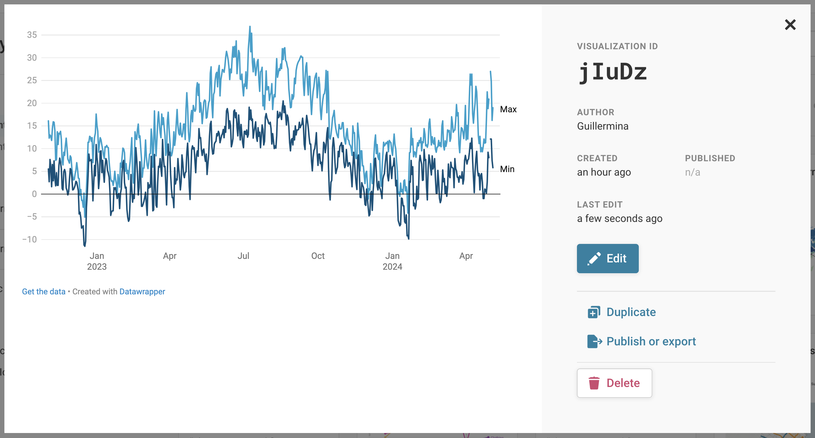
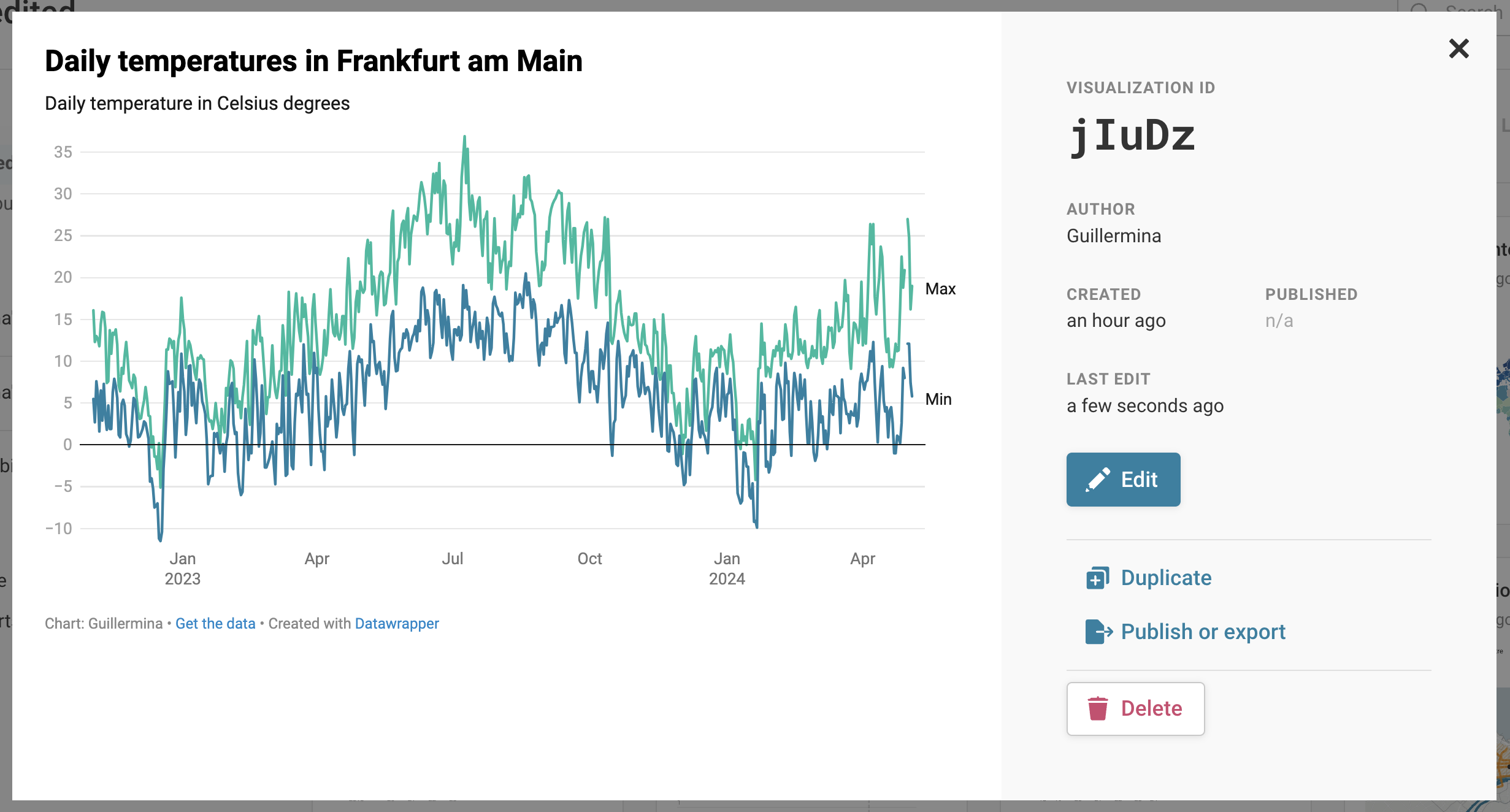
If you log into your Datawrapper account and you should be able to see the new chart you just created in your Archive. It should look something like this:

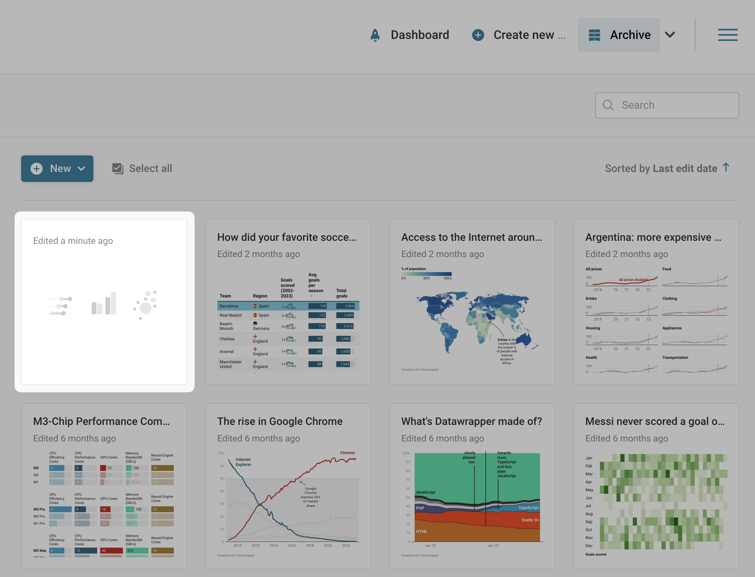
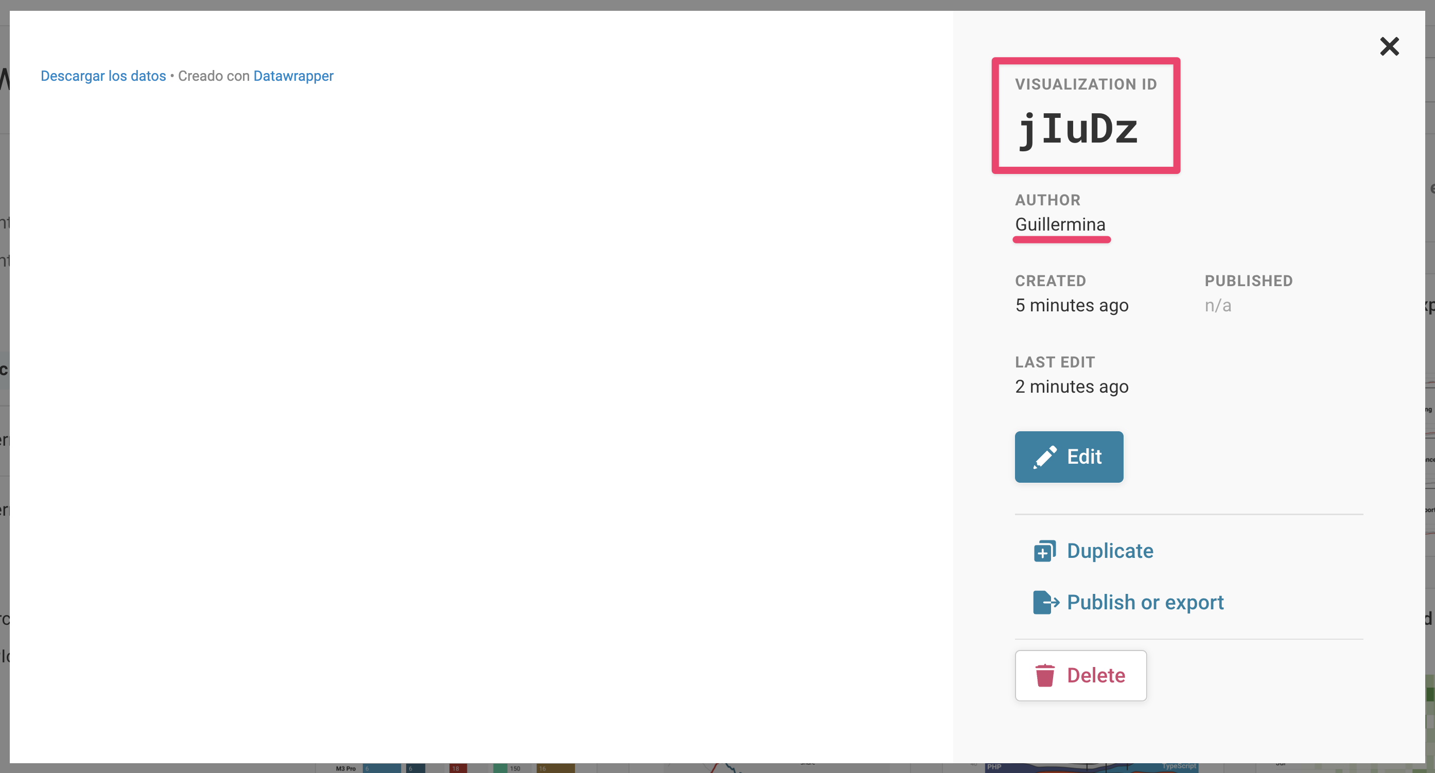
If you click on it, you can access more chart details e.g. chart ID, author, a timestamp for when it was created, last edited and published. All this should match the information that the dw_create_chart() returned in the RStudio console when we ran it!

Downloading the data

Good! You created a line chart, but you may have noticed that the line chart is blank. It’s empty because you haven’t added data to it. Yet. Let’s do that then!

The data in this tutorial come from the German Weather Service (DWD) and uses the rdwd package to access it in R.

📘

Go over the documentation of a package before using it.

This will help you to have an overview of what the package does and will give you detailed information about the functions and arguments that you can pass to each function.

In the next steps, you’ll use the functions in rdwd to retrieve and clean daily data for min and max temperatures in Frankfurt/Main , one of the biggest cities in Western Germany.

The first step is to use the selectDWD() function to select the dataset. Select last year’s daily climate data from Frankfurt am Main and save the output in a variable called frankfurt:

# select a dataset 
frankfurt <- selectDWD("Frankfurt/Main", res="daily", var="kl", per="recent")

To actually download these data and read it, do the following:

# download that dataset  
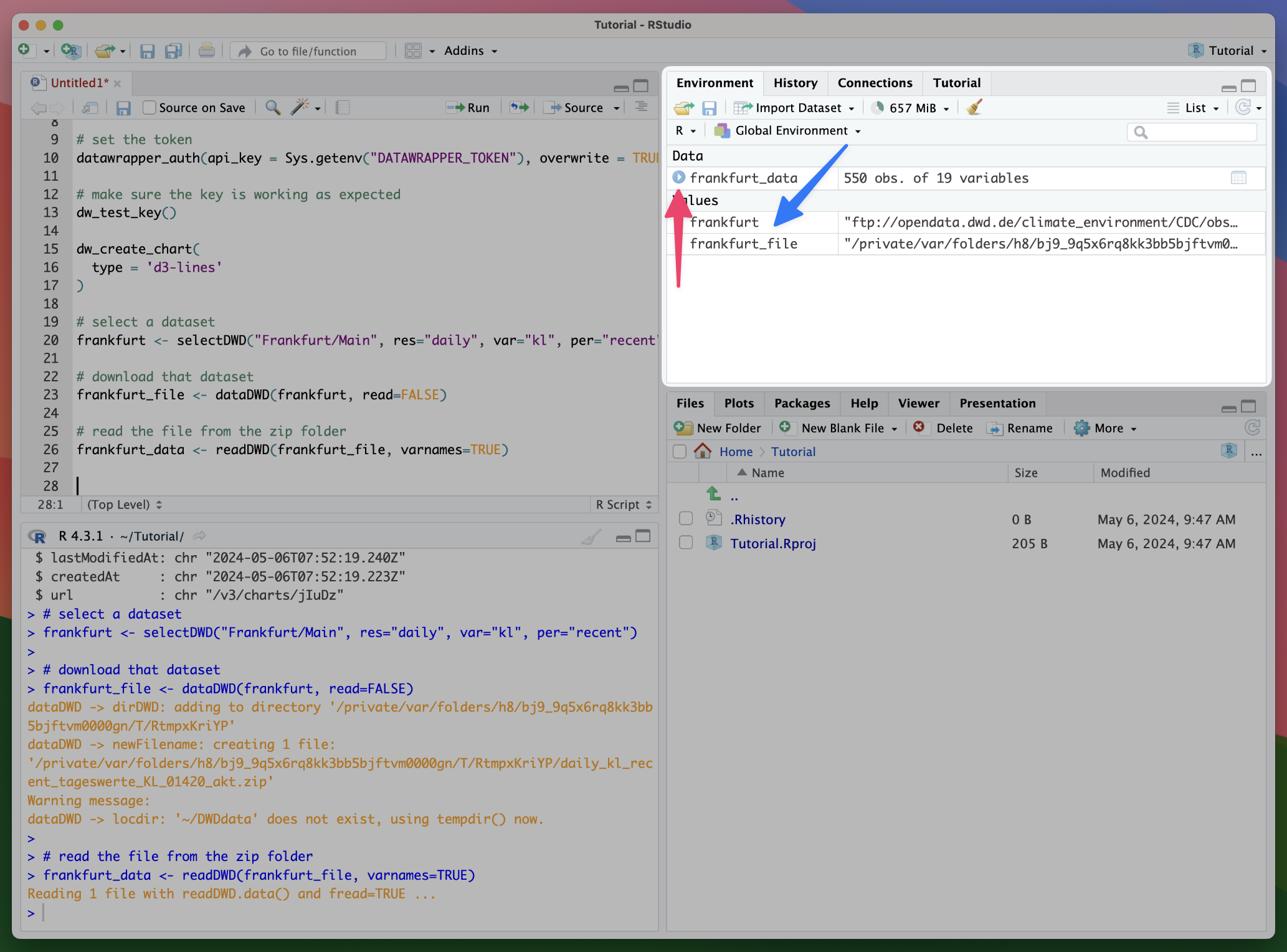
frankfurt_file <- dataDWD(frankfurt, read=FALSE)    
	
# read the file from the zip folder  
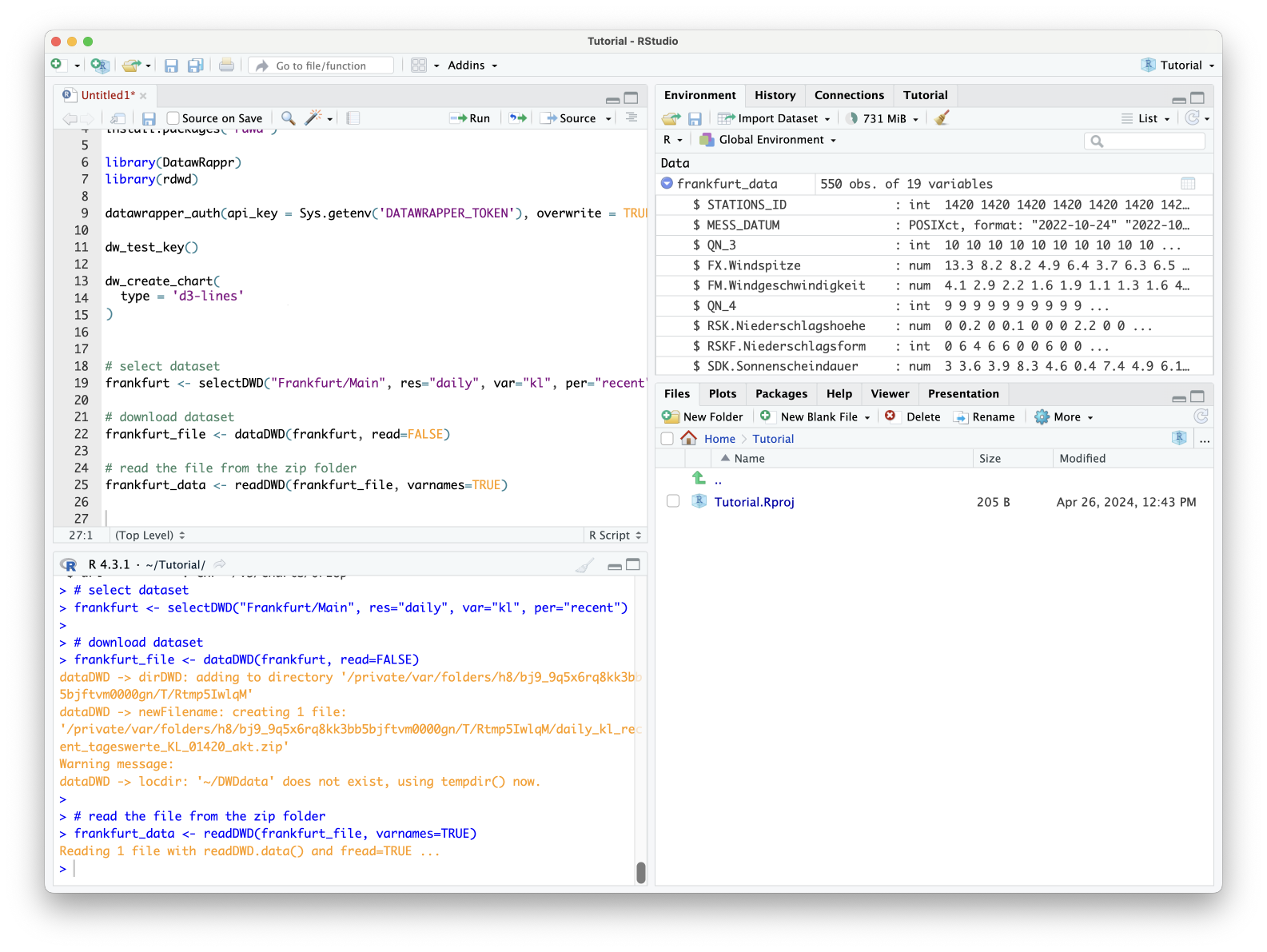
frankfurt_data <- readDWD(frankfurt_file, varnames=TRUE)

You’ll notice in the Environment tab that frankfurt and frankfurt_file have been successfully saved and are now listed there. frankfurt_data is the name of the dataset we selected and you can explore it further (look at the names of the columns, number of rows, etc.) if you click on the ▶️ right next to it in the Environment tab in RStudio:

Preparing the data

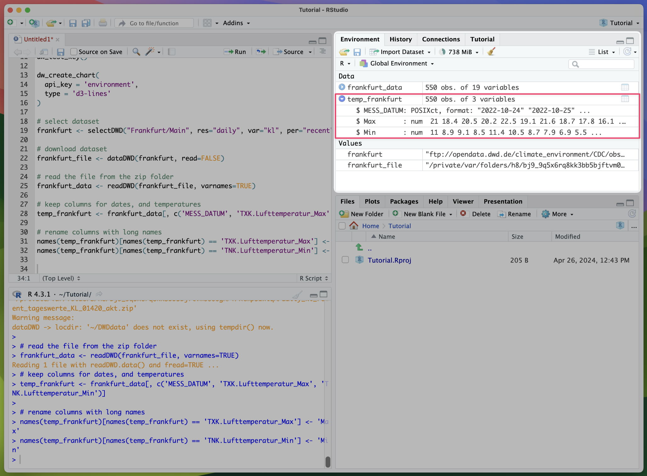
For this chart, let’s show the daily development of the min and max temperatures in Frankfurt am Main. To do this, select the columns with the date, max and min temperatures ('MESS_DATUM', 'TXK.Lufttemperatur_Max', 'TNK.Lufttemperatur_Min', respectively) from the dataset. You’re probably noticing how long the names of the temperature columns are. Let’s rename them!

• 'TXK.Lufttemperatur_Max' → 'Max'
• 'TNK.Lufttemperatur_Min' → 'Min'

# keep columns for dates, and temperatures
temp_frankfurt <- frankfurt_data[, c('MESS_DATUM', 'TXK.Lufttemperatur_Max', 'TNK.Lufttemperatur_Min')]  

# rename columns with long names
names(temp_frankfurt)[names(temp_frankfurt) == 'TXK.Lufttemperatur_Max'] <- 'Max'  
names(temp_frankfurt)[names(temp_frankfurt) == 'TNK.Lufttemperatur_Min'] <- 'Min'

After cleaning the data and running the code, you’ll notice that a new clean dataset with the daily values for min and max temperatures in Frankfurt am Main appears in the Environment tab in RStudio. Good! You’re ready to move to the next step!

📘

Why you should clean your data before uploading it into Datawrapper

Datawrapper is intended to cover the “last step” in the data visualization process. It’s not intended to do data analysis or column operations like you would do in some BI tools. One should do all the data cleaning before uploading or pushing data into Datawrapper. And because you won’t be loading data that it’s not being visualized, this will improve the performance of the chart.

💡 As a hint, click on the "R" tab to reveal the code up until this point.

# install packages
install.packages('devtools')
devtools::install_github('munichrocker/DatawRappr')
install.packages('rdwd')

library(DatawRappr)
library(rdwd)

# create an environment for the token 
# (after you run it, you can delete this line) 
Sys.setenv(DATAWRAPPER_TOKEN = "your token goes here")

# set the token
datawrapper_auth(api_key = Sys.getenv("DATAWRAPPER_TOKEN"), overwrite = TRUE)

# make sure the key is working as expected
dw_test_key()

# create line chart
dw_create_chart(  
	api_key = 'environment',      
	type = 'd3-lines'
)

# select a dataset 
frankfurt <- selectDWD("Frankfurt/Main", res="daily", var="kl", per="recent")

# download that dataset  
frankfurt_file <- dataDWD(frankfurt, read=FALSE)    
	
# read the file from the zip folder  
frankfurt_data <- readDWD(frankfurt_file, varnames=TRUE)

# keep columns for dates, and temperatures
temp_frankfurt <- frankfurt_data[, c('MESS_DATUM', 'TXK.Lufttemperatur_Max', 'TNK.Lufttemperatur_Min')]  

# rename columns with long names
names(temp_frankfurt)[names(temp_frankfurt) == 'TXK.Lufttemperatur_Max'] <- 'Max'  
names(temp_frankfurt)[names(temp_frankfurt) == 'TNK.Lufttemperatur_Min'] <- 'Min'

Exploring the chart metadata

Now that you have cleaned the data, you’ll need to “upload” it into the empty line chart. DatawRappr has a function that will help you with that. dw_data_to_chart() lets you fill a chart with some data. From the documentation, you’ll notice that this function needs x (data) and the line chart ID as arguments. Remember that the chart ID here will be the one you got after running dw_create_chart() when you first created the line chart.

# add data to line chart
dw_data_to_chart(    
		temp_frankfurt,    
		chart_id = "YOUR CHART ID"  
	)

If you run the code, the console should return a success message like: Data in [YOUR CHART ID] successfully updated. If you also look at the preview of the line chart in your Datawrapper Archive on the web app, you’ll see that it has been updated and it’s now showing the min and max temperatures!

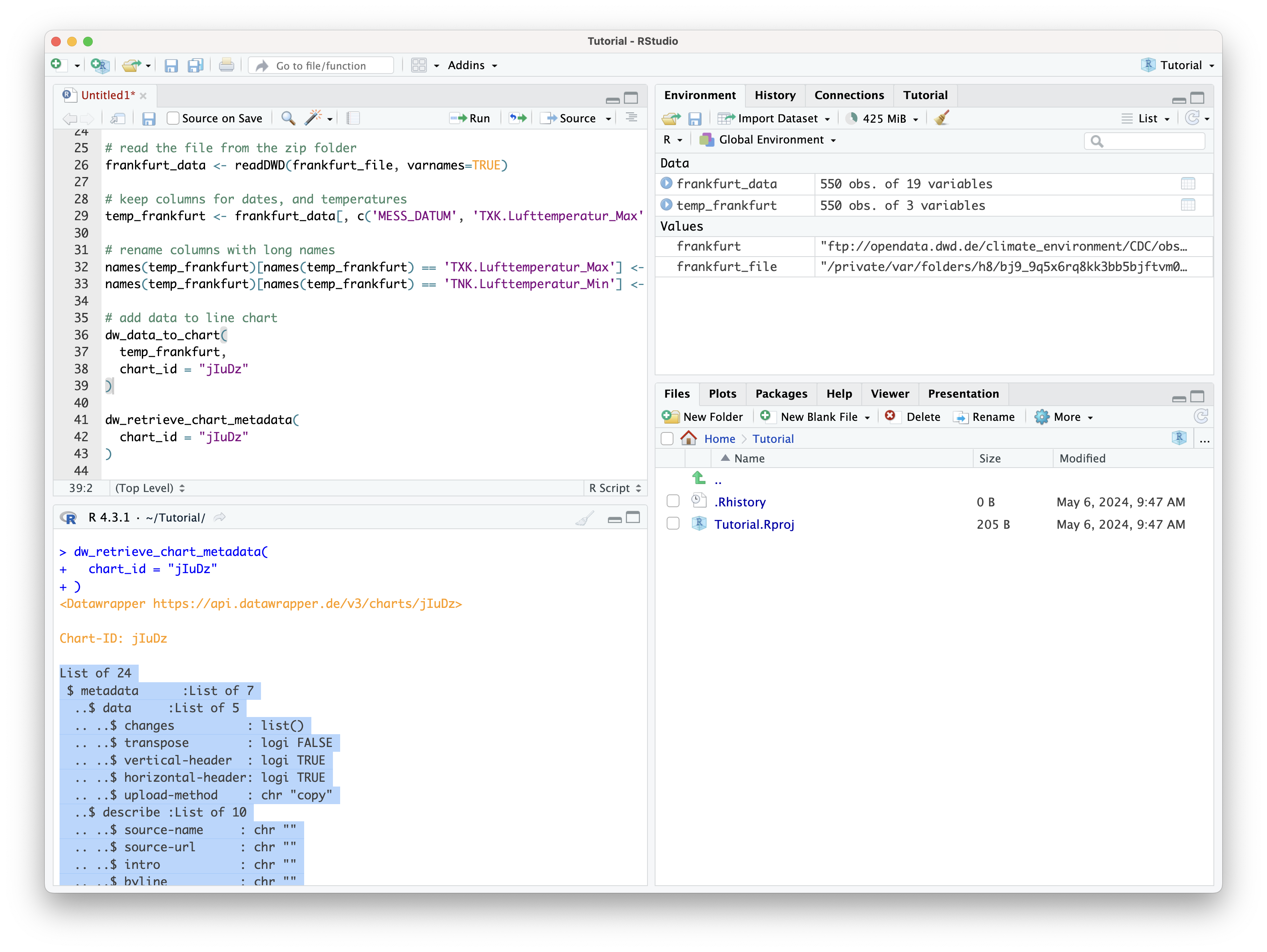
You can take a closer look at the metadata (content or information) of the chart using the dw_retrieve_chart_metadata() function. If you pass the chart ID and run it, it will return all the metadata from the chart. As the author of the DatawRappr package Benedict Witzenberger states in the docs, this function “is helpful to gain insights in the different options that might be changed via the API.” Any changes you make to the chart, will be reflected in the metadata and you’ll always have access to it with dw_retrieve_chart_metadata().

Another way of looking at the metadata, is by going to https://api.datawrapper.de/v3/charts/[YOUR CHART ID]. If you download this JSON formatter (a Google Chrome extension to make JSON files easier to read), this is what it should look like:

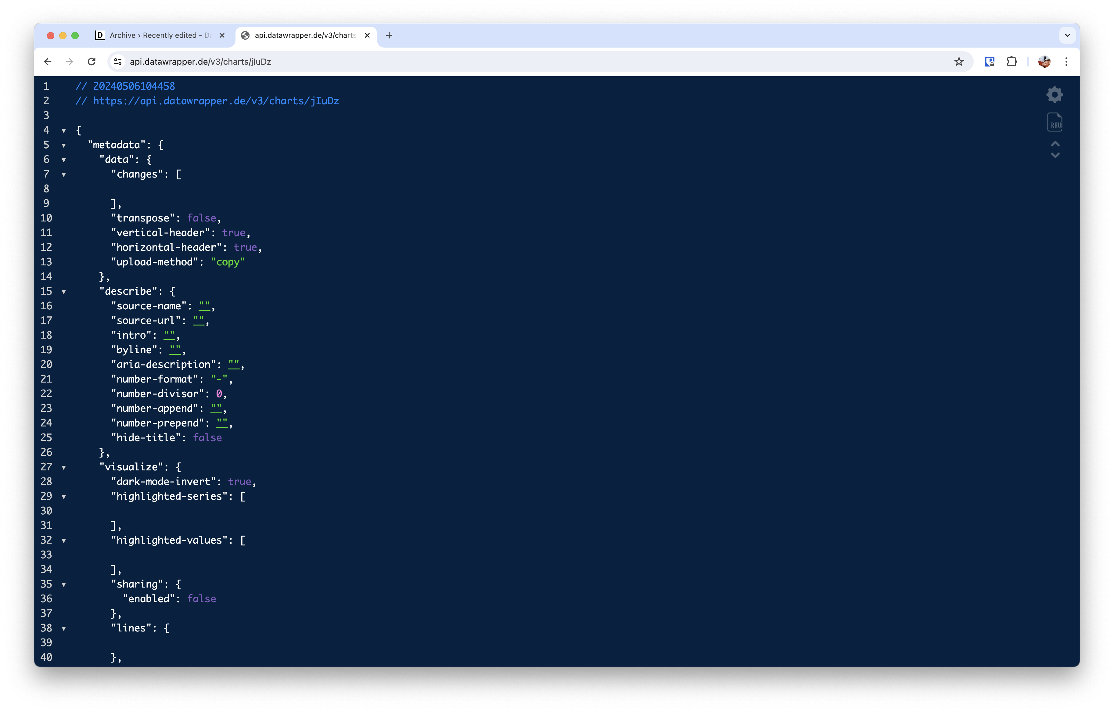
If you take a closer look at the chart information, you can notice that under "describe" there are lots of empty fields such as "source-name", "intro", "byline", etc. All these fields are aspects of the line chart that you can directly edit on the web app.

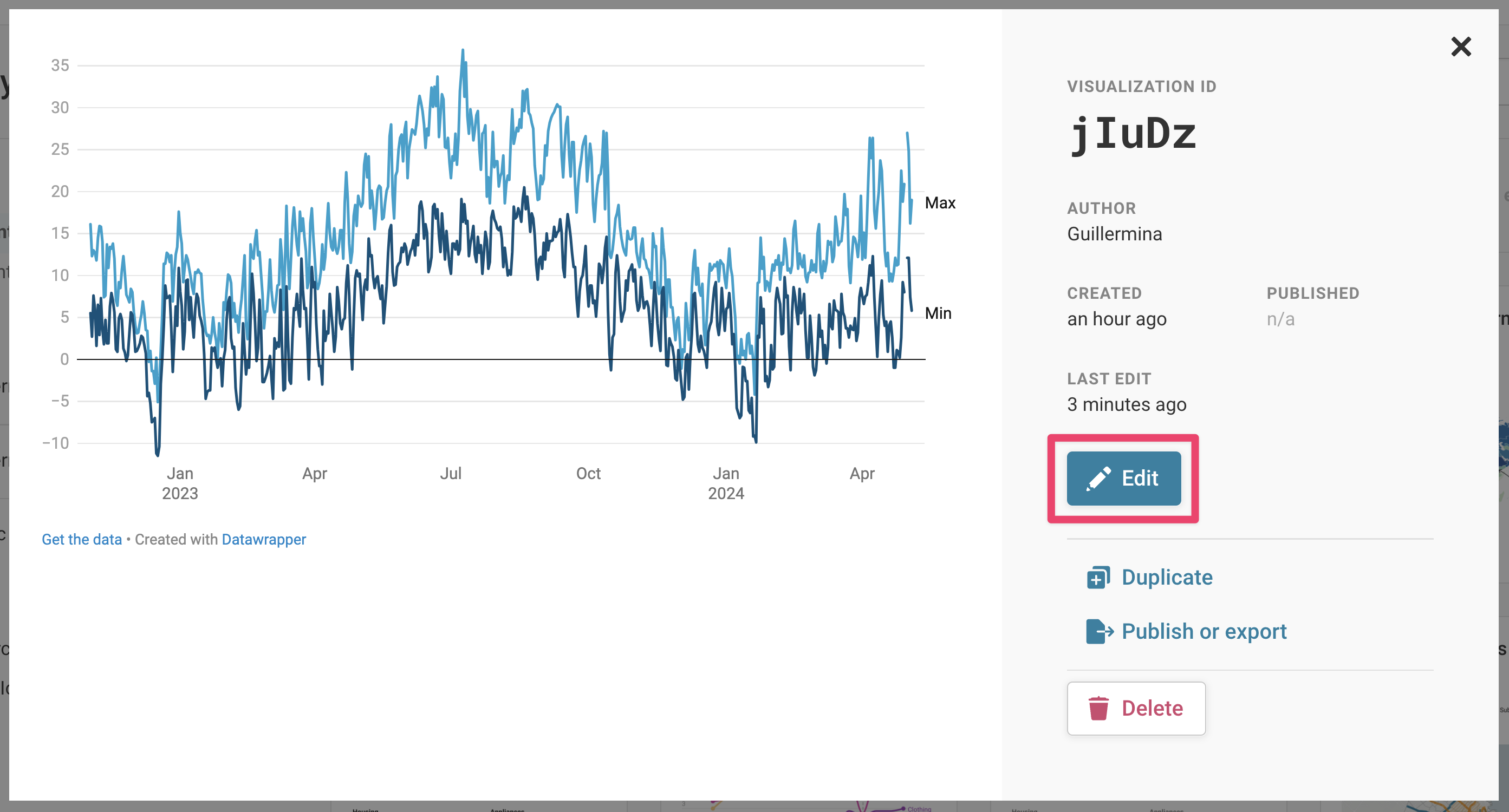
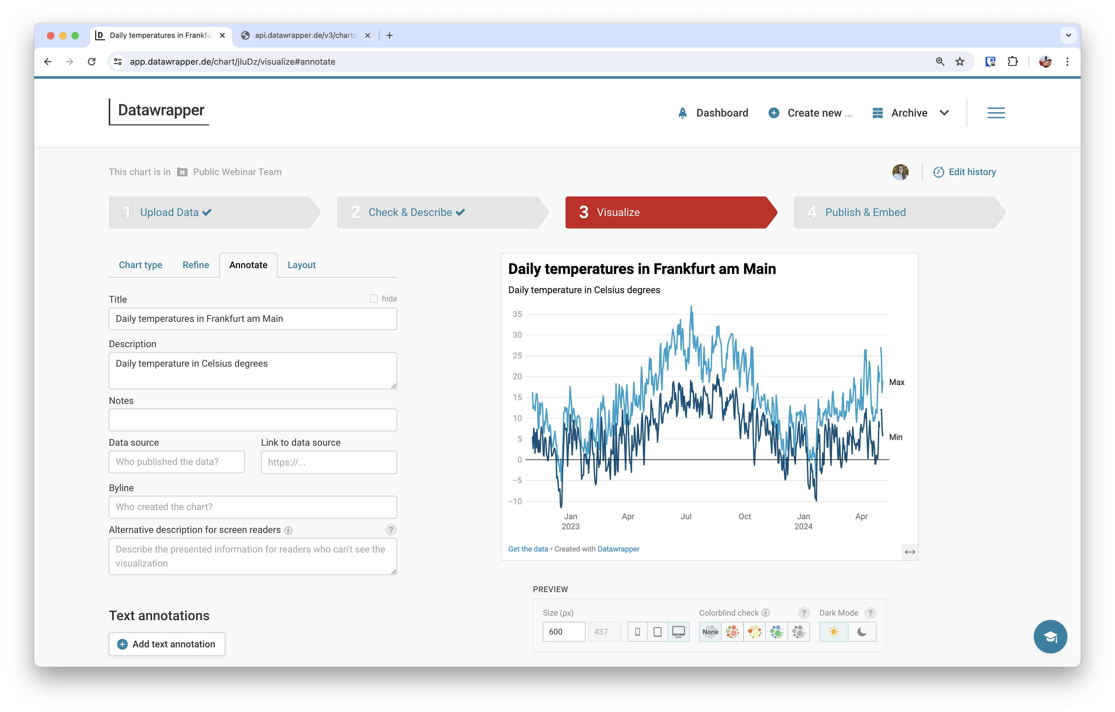
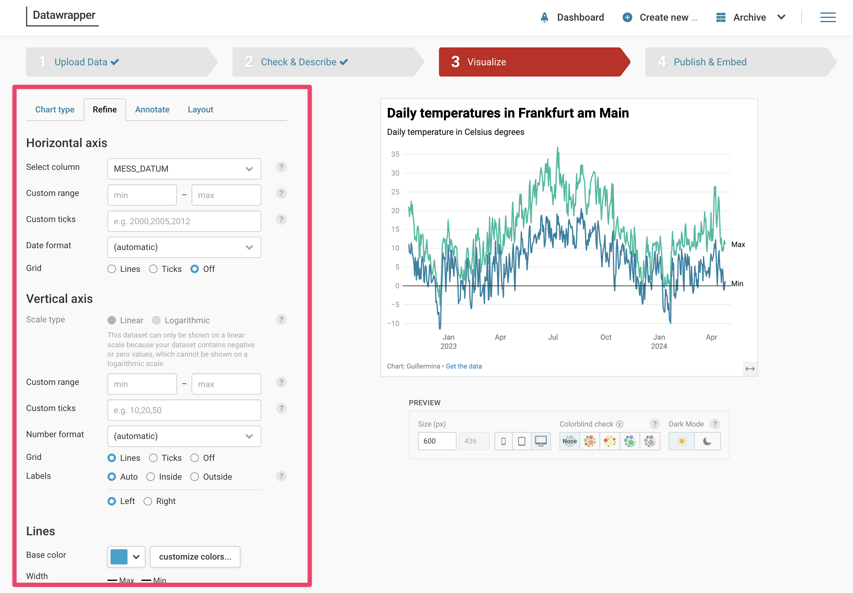
If you go back to your Datawrapper Archive and click on Edit in the line chart preview, you’ll be able to access the chart editor:

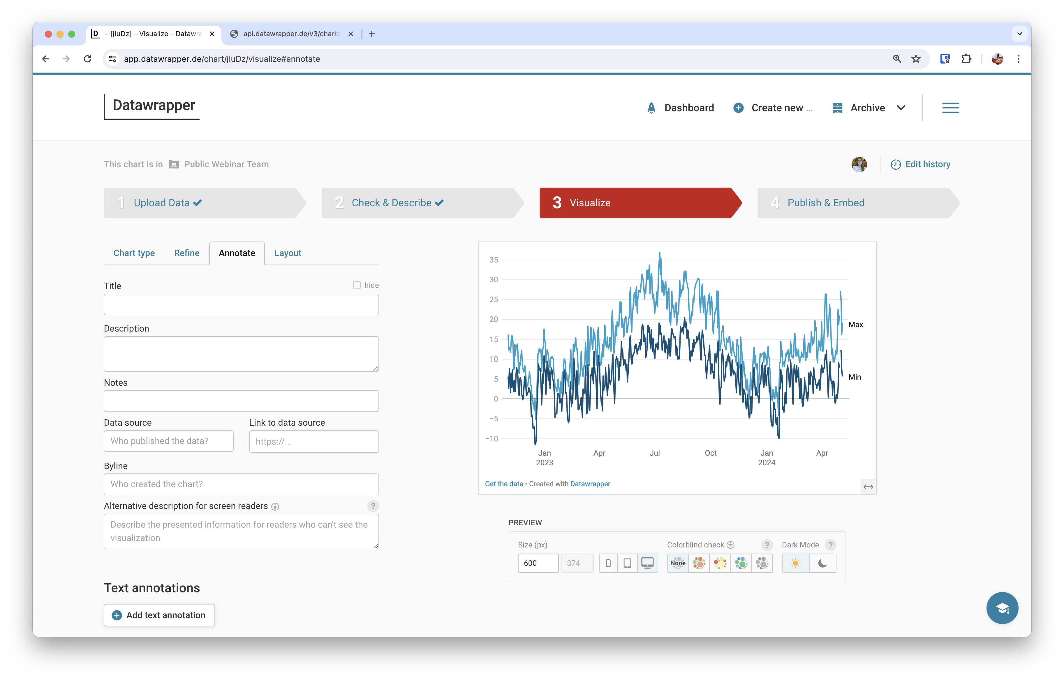
At the top of the chart editor you’ll notice all the steps you need to take in Datawrapper to create a chart. If you click on Upload Data, you’ll see the temperature data for Frankfurt am Main that we uploaded through the API. The Check & Describe step will show you information on the column type (numerical, dates, etc.), among others. The Visualize step is where you can keep editing your chart by changing the colors of the lines, for example, or adding a title and a description. All the changes you make here, will be reflected on the chart metadata ⬇️

Let’s add a title, a description and a byline on the chart editor and see how these changes reflect on https://api.datawrapper.de/v3/charts/[YOUR CHART ID] .

If you now go back to https://api.datawrapper.de/v3/charts/[YOUR CHART ID] and refresh the page, you’ll notice that the chart metadata has updated to reflect these changes.

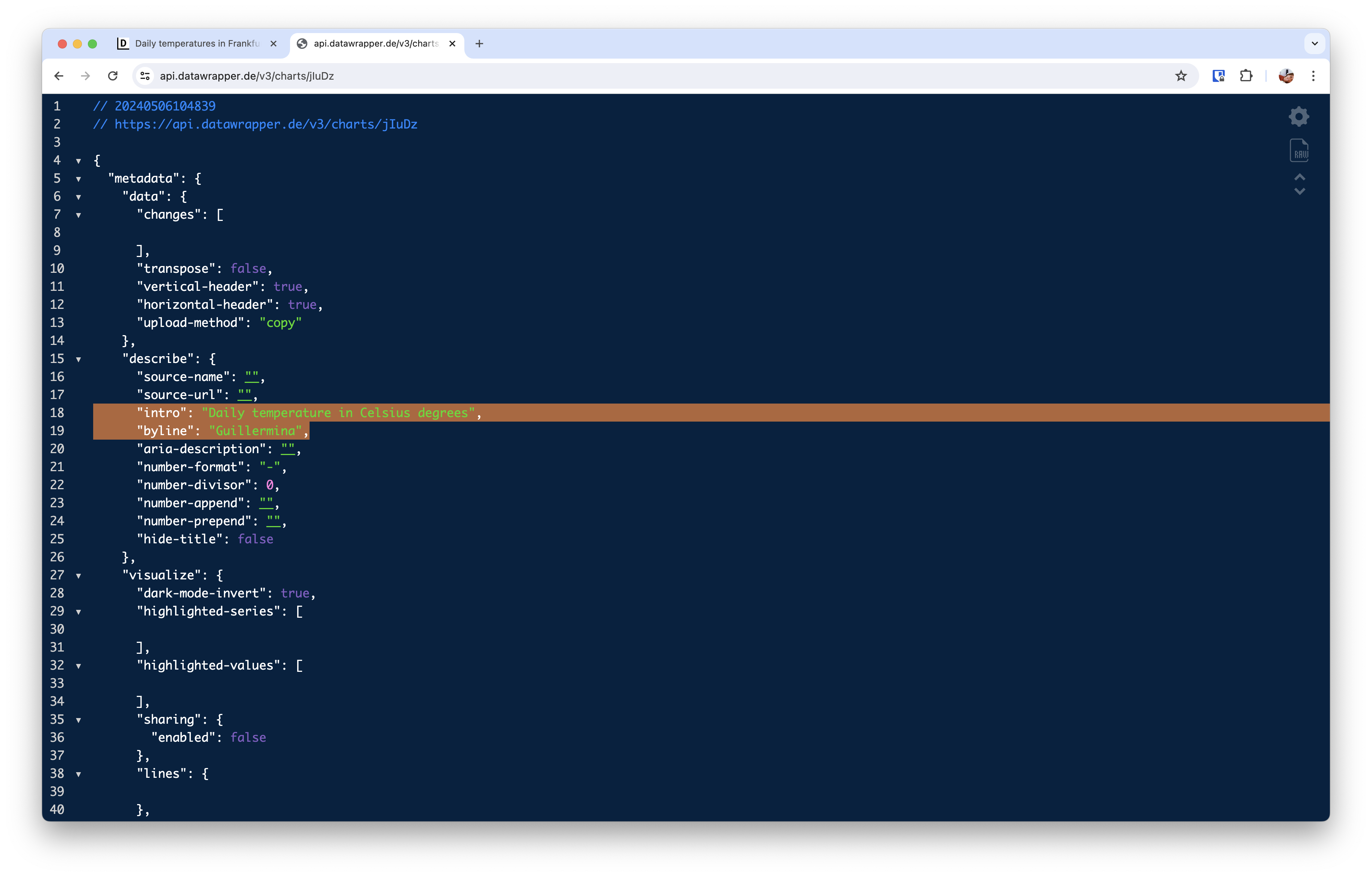
The same will be true if you now run dw_retrieve_chart_metada() again in RStudio. You should see these changes reflected in .. ..$ intro: "Daily temperature in Celsius degrees" below ..$ describe :List of 10.

Editing the chart

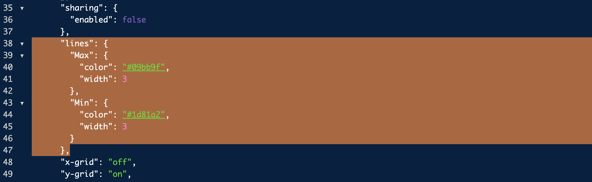
The same way you updated the chart through the web app, you can do it through RStudio. For example, let’s try to change the color of the lines. You’ll be able to do this with the dw_edit_chart() function. From the documentation, you’ll see that this function needs the chart ID as an argument (so that Datawrapper knows which chart we want to edit) and the specific colors for each line in your line chart (the Max and Min lines). You can color the lines using the following HEX codes: #09bb9f and #1d81a2 for each line, respectively, like this:

# edit chart
dw_edit_chart(  
	chart_id = "YOUR CHART ID",    
	
	visualize = list(              
		lines = list(                    
			'Max' = list(        
				color = '#09bb9f'      
			),      
			
			'Min' = list(        
				color = '#1d81a2'      
			)    
		)    
	)
)

After you run it, you’ll see a success message in the console that reads: Chart [YOUR CHART ID] succesfully updated. Now, if you head to https://api.datawrapper.de/v3/charts/[YOUR CHART ID] and refresh it, you’ll see these changes were successfully implemented:

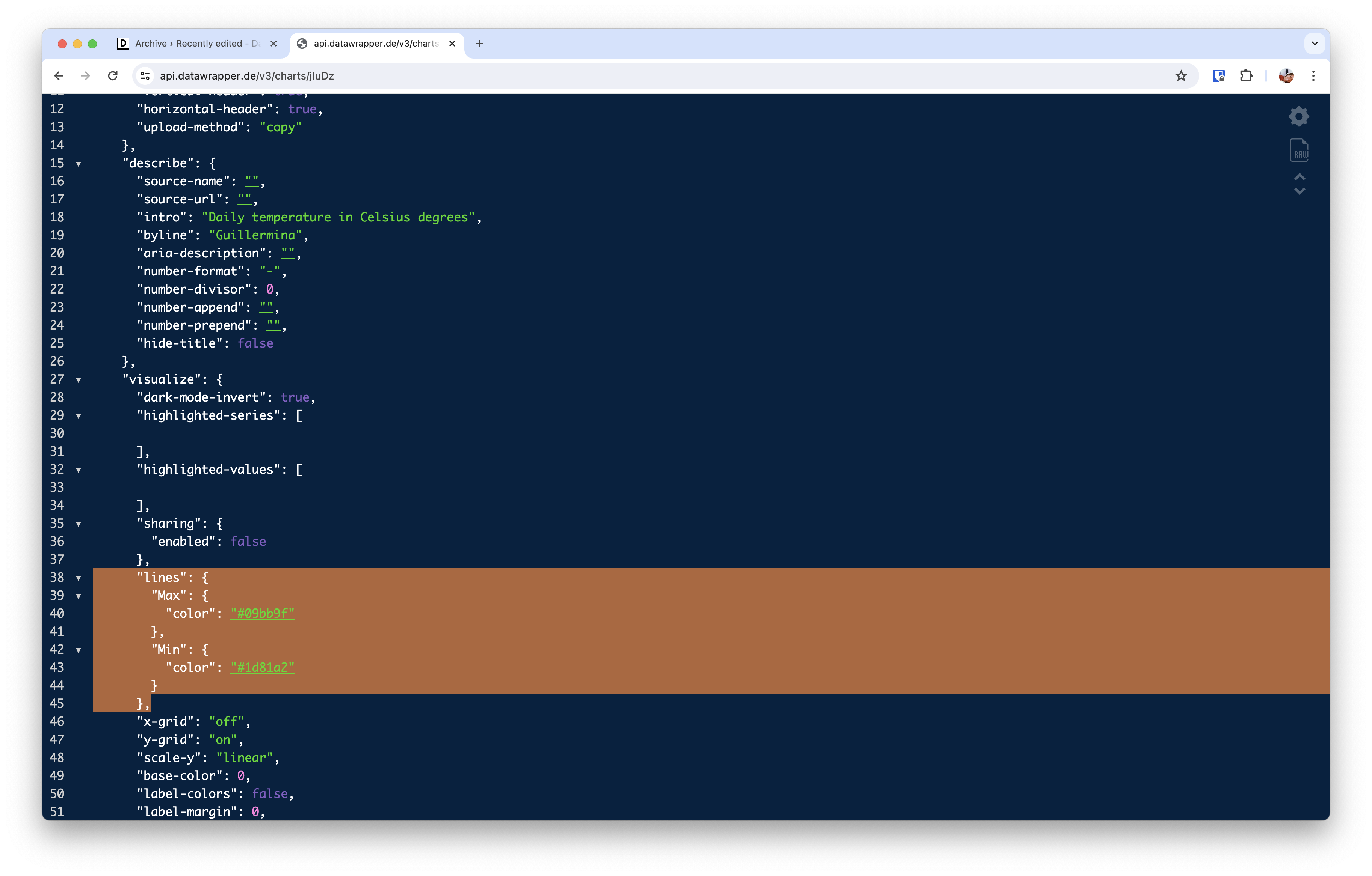
If you head to your Datawrapper Archive and click on the chart preview, you’ll also see the updated line chart with the new colors.

⭐

Bonus points for...

Can you spot these changes if you run dw_retrieve_chart_metadata() again in RStudio?

💡 As a hint, click on the "R" tab to reveal the code up until this point.

# install packages
install.packages('devtools')
devtools::install_github('munichrocker/DatawRappr')
install.packages('rdwd')

library(DatawRappr)
library(rdwd)

# create an environment for the token 
# (after you run it, you can delete this line) 
Sys.setenv(DATAWRAPPER_TOKEN = "your token goes here")

# set the token
datawrapper_auth(api_key = Sys.getenv("DATAWRAPPER_TOKEN"), overwrite = TRUE)

# make sure the key is working as expected
dw_test_key()

# create line chart
dw_create_chart(  
	api_key = 'environment',      
	type = 'd3-lines'
)

# select a dataset 
frankfurt <- selectDWD("Frankfurt/Main", res="daily", var="kl", per="recent")

# download that dataset  
frankfurt_file <- dataDWD(frankfurt, read=FALSE)    
	
# read the file from the zip folder  
frankfurt_data <- readDWD(frankfurt_file, varnames=TRUE)

# keep columns for dates, and temperatures
temp_frankfurt <- frankfurt_data[, c('MESS_DATUM', 'TXK.Lufttemperatur_Max', 'TNK.Lufttemperatur_Min')]  

# rename columns with long names
names(temp_frankfurt)[names(temp_frankfurt) == 'TXK.Lufttemperatur_Max'] <- 'Max'  
names(temp_frankfurt)[names(temp_frankfurt) == 'TNK.Lufttemperatur_Min'] <- 'Min'

# add data to line chart
dw_data_to_chart(      
	temp_frankfurt,      
	chart_id = "YOUR CHART ID"  
)

# retrieve chart metadata
dw_retrieve_chart_metadata(  
	chart_id = "YOUR CHART ID"
)

# edit chart
dw_edit_chart(  
	chart_id = "YOUR CHART ID",    
	
		visualize = list(              
		lines = list(                    
			'Max' = list(        
				color = '#09bb9f'
			),      
			
			'Min' = list(        
				color = '#1d81a2'
			)    
		)    
	)
)

Changing the colors of the lines is just one of the maaaany options available to edit the line chart. All the customization options you see on left side of the screen in the Visualize step in the web app, you can edit them through the API in RStudio. You can always refer back to the DatawRappr documentation and Datawrapper’s API documentation to learn more about each chart property and how to customize it.

I recommend you try a few on your end to get a better sense of how it works. Here’s what you can try:

⭐

Bonus points for...

Can you change the width of the lines?

Hint: you can use the 'width' property just like you did before with 'color' and pass a number to set the width the width of the line for both 'Min' and 'Max' temperature

R

visualize = list(  
   lines = list(  
     LINE 1 = list(  
        PROPERTY 1, PROPERTY 2, ANOTHER PROPERTY),  
     LINE 2 = list(  
        PROPERTY 1, PROPERTY 2, ANOTHER PROPERTY)  
     )  
   )  
)

where the properties are 'color' and 'width', for example.

Don’t forget to check https://api.datawrapper.de/v3/charts/[YOUR CHART ID] to see if your changes were implemented in the line chart. It should look like this:

💡 As a hint, click on the "R" tab to reveal the code up until this point.

# install packages
install.packages('devtools')
devtools::install_github('munichrocker/DatawRappr')
install.packages('rdwd')

library(DatawRappr)
library(rdwd)

# create an environment for the token 
# (after you run it, you can delete this line) 
Sys.setenv(DATAWRAPPER_TOKEN = "your token goes here")

# set the token
datawrapper_auth(api_key = Sys.getenv("DATAWRAPPER_TOKEN"), overwrite = TRUE)

# make sure the key is working as expected
dw_test_key()

# create line chart
dw_create_chart(  
	api_key = 'environment',      
	type = 'd3-lines'
)

# select a dataset 
frankfurt <- selectDWD("Frankfurt/Main", res="daily", var="kl", per="recent")

# download that dataset  
frankfurt_file <- dataDWD(frankfurt, read=FALSE)    
	
# read the file from the zip folder  
frankfurt_data <- readDWD(frankfurt_file, varnames=TRUE)

# keep columns for dates, and temperatures
temp_frankfurt <- frankfurt_data[, c('MESS_DATUM', 'TXK.Lufttemperatur_Max', 'TNK.Lufttemperatur_Min')]  

# rename columns with long names
names(temp_frankfurt)[names(temp_frankfurt) == 'TXK.Lufttemperatur_Max'] <- 'Max'  
names(temp_frankfurt)[names(temp_frankfurt) == 'TNK.Lufttemperatur_Min'] <- 'Min'

# add data to line chart
dw_data_to_chart(      
	temp_frankfurt,      
	chart_id = "YOUR CHART ID"  
)

# retrieve chart metadata
dw_retrieve_chart_metadata(  
	chart_id = "YOUR CHART ID"
)

# edit chart
dw_edit_chart(  
	chart_id = "YOUR CHART ID",    
	
		visualize = list(              
		lines = list(                    
			'Max' = list(        
				color = '#09bb9f',
				**width = 3**      
			),      
			
			'Min' = list(        
				color = '#1d81a2',
				**width = 3**      
			)    
		)    
	)
)

Publishing

Now that you’ve made these edits, you’ll probably want to publish the line chart. To do this, you can use the dw_publish_chart() function. It takes the chart ID as argument and, optionally, we can also ask the function to return the code for the responsive iFrame and an URL to the chart.

# publish the chart
dw_publish_chart(      
	chart_id = "YOUR CHART ID",      
	return_urls = TRUE  
)

After running it, you should see a success message Chart [YOUR CHART ID] published! followed by the code for the responsive iFrame and the chart URL.

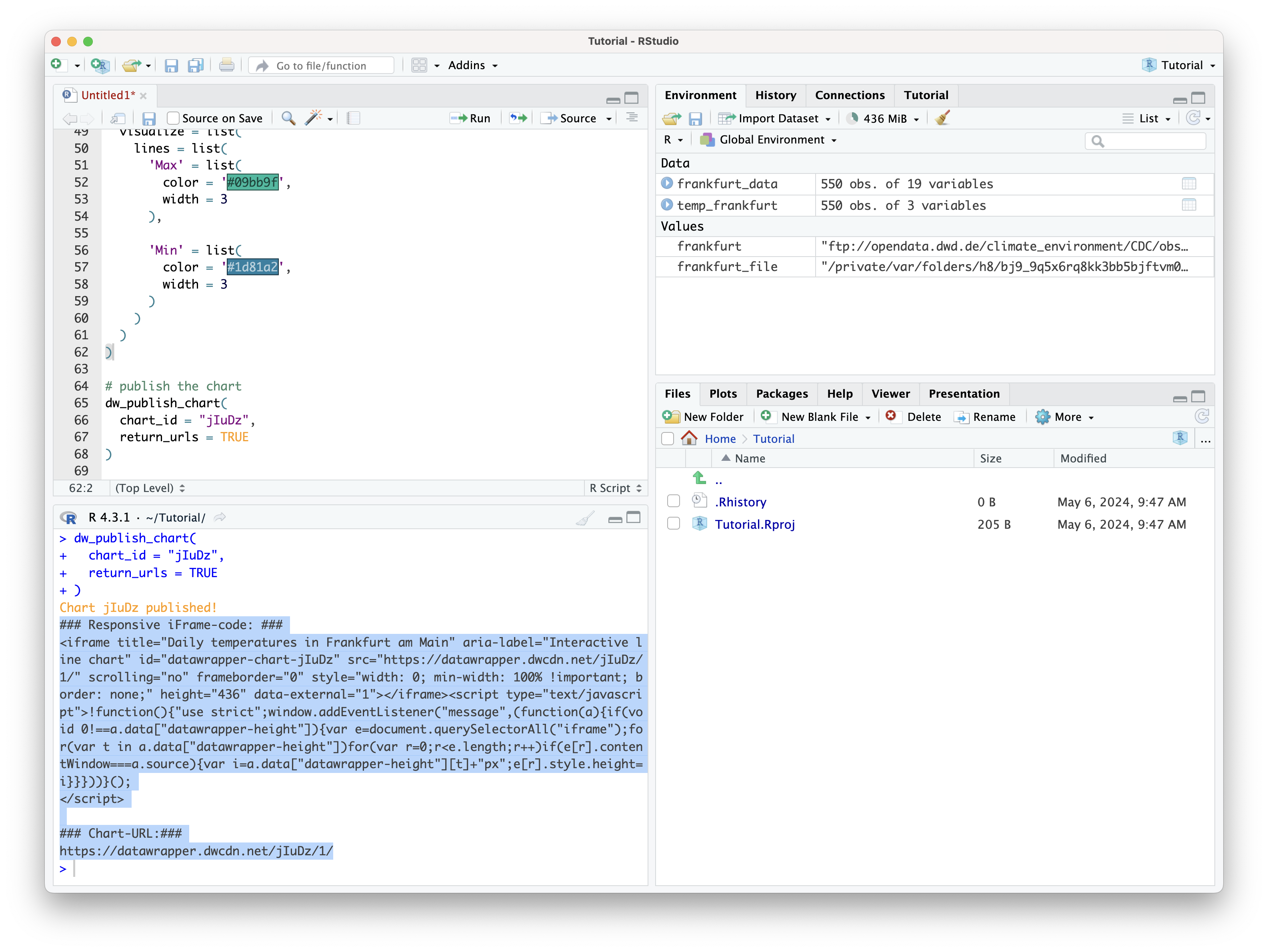
Congrats! You just published a chart through RStudio using Datawrapper’s API! 🤩

Publishing one chart is just scratching the surface of what you can do with Datawrapper’s API in RStudio. What you saw in this tutorial is just the starting point. From this point onwards, you’ll be able to dive even deeper… Can you think of some practical applications for the API? For example, imagine creating several line charts, all with the same style, but showing the temperatures of different cities in Germany… The possibilities are endless!

Resources

Here are some useful resources you can always refer to along your journey with Datawrapper’s API:

• Unwrapped: Datawrapper API → a collection of talks from Datawrapper’s conference Unwrapped, where users share tips, how to's, and different ways they use Datawrapper’s API.
• The official DatawRappr (package docs)
• Guest post by the DatawRappr package creator Benedict Witzenberger: Why I created an R package to use Datawrapper’s API and how to use it
• Anouncement of the Datawrapper API: Automate your chart creation with our new API

If you ever run into any questions, you can always reach out to us at [email protected]

Happy charting! 📈